 ReliCheck Quanta · Plain-English Teaching Guide
One-Way ANOVA · Worked Example
ReliCheck Quanta · Plain-English Teaching Guide
One-Way ANOVA · Worked Example
 Teaching Guide 01
Understanding ANOVA
What these numbers say — a one-way ANOVA read start to finish in Quanta
Explained from scratch for readers who have never taken a statistics course.
You do not need any statistics background. Every term is defined the first time it shows up, in plain words, right before you need it. Work through it once with the software open and you will be able to read an ANOVA screen and say what it means.
The whole guide follows one real analysis in Quanta: does Job Performance Score differ across Role Level, using a sample of 250 people. Watch that one question get answered, number by number.
In plain terms, Role Level does not clearly move Job Performance in this sample. The rest of this guide unpacks what every piece of that line means and how the software got there.
What is ANOVA, really?
ANOVA is short for Analysis of Variance. Set the name aside for a second and picture the actual problem. You have one number you care about for each person (here, a job performance score). You have people sorted into a few groups (here, five role levels). You want to know one thing: do the groups score about the same on average, or does at least one group stand apart?
You could just eyeball the group averages. The trouble is that averages always differ a little by luck, even when nothing real is going on. Pull five random handfuls of people from the same room and their average heights will not be identical. ANOVA is the tool that separates a real gap between groups from the ordinary luck-of-the-draw wobble you would expect anyway.
Signal is how far apart the group averages sit. Noise is how much people bounce around inside their own group. ANOVA compares the two. When the signal is large next to the noise, the groups probably differ for real. When the signal is small next to the noise, the gaps you see are the kind luck produces on its own.
That single comparison, signal measured against noise, is the whole idea. Every number on the screen is a way of sizing it up.
What are we asking the data?
Write the question in words before the software computes anything:
Do average Job Performance Scores differ across Role Level in this sample?
Notice what the question does not say. It does not say role causes performance. It does not say which two roles differ. One question comes first: is there any between-role difference worth noticing at all. You earn the follow-up questions only after this one clears the bar.
Two ideas you need here
Statistics starts by assuming nothing is going on, then measures whether the data give enough reason to drop it. The “nothing going on” version here is: all five role levels have the same true average job performance. That assumption is the null hypothesis. ANOVA measures how much the data count against it. If the push is strong enough, you reject the null and conclude the averages really do differ.
With five role levels there are ten possible pairs to compare (Manager vs. Team lead, Manager vs. Director, and so on). A t-test compares two groups at a time. Run all ten and you give yourself ten chances to stumble onto a “significant” gap by luck, which badly inflates the odds of a false alarm. ANOVA asks one combined question first: is anything different anywhere? Only if that clears the bar do you go hunting for which pairs are responsible.
How you set it up in Quanta
- 01Open MM Test Emotional_Intelligence_QuanHeavy.xlsx and confirm all 250 cases load cleanly.
- 02In the sidebar go to Evidence → Compare Means → One-way ANOVA (the Group Patterns screen).
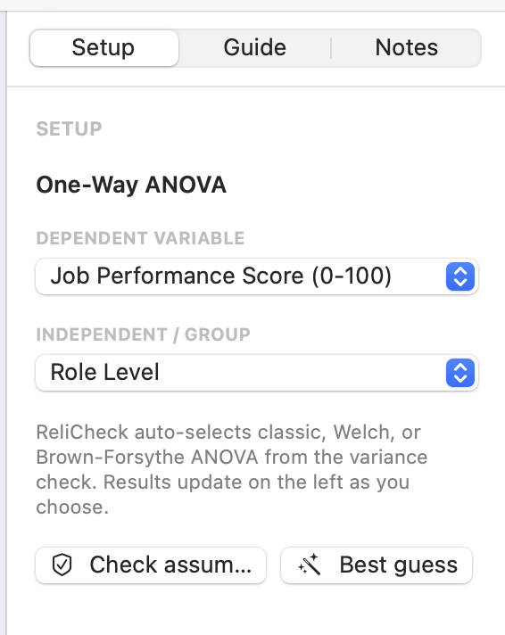
- 03In the right panel set Dependent = Job Performance Score (0–100) and Independent / group = Role Level.
- 04Results fill in on the left as you choose. On this path there is no separate Run button.
The setup panel is where you define the analysis: which column is the outcome you are explaining, and which column splits people into groups. Quanta picks the specific model (classic ANOVA, Welch, or Brown-Forsythe) from an automatic variance check, so you are not choosing the model out of habit. The Check assumptions button runs the safety tests (more on those in Lesson 3) before you rely on the result.
Five role levels. One person belongs to one role. Performance runs on a 0 to 100 scale. If role level mattered a lot for performance here, the five averages would separate cleanly, and by a wide margin next to the scatter inside each role. Keep that mental picture. The numbers either confirm it or they do not.
Read the headline numbers as a verdict on this sample
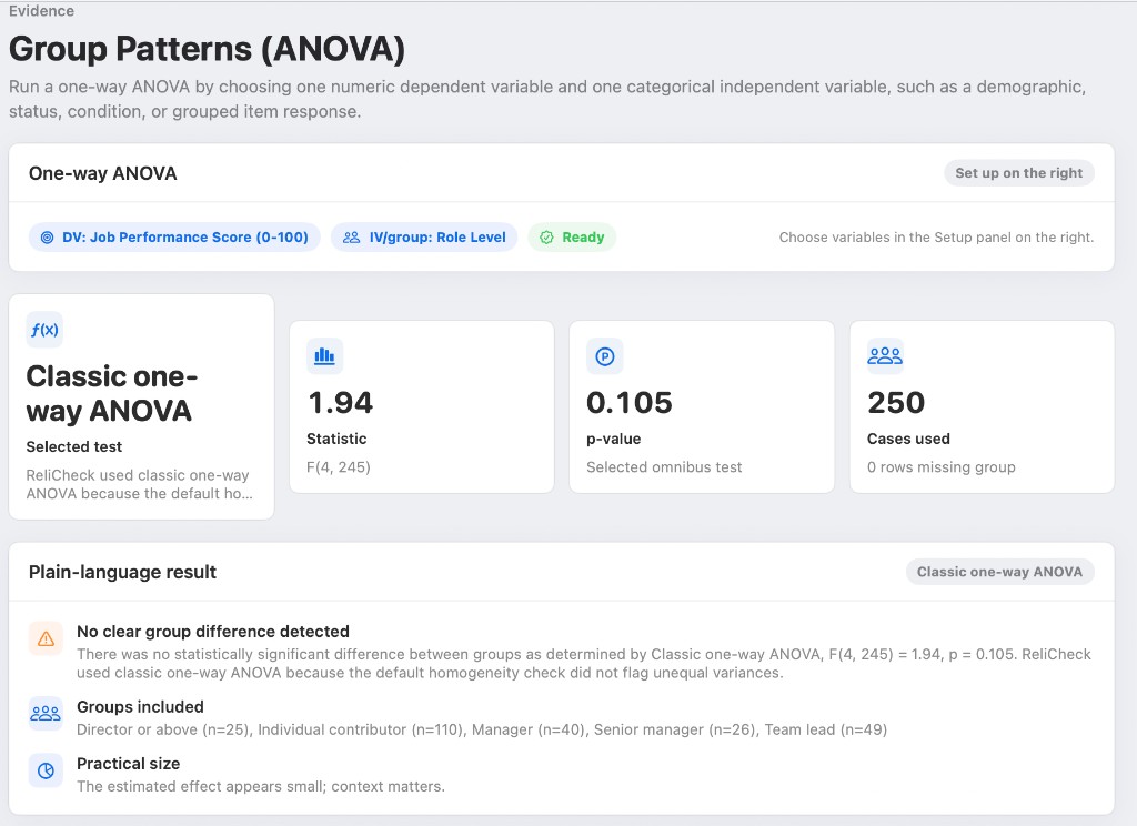
What each tile is telling you
- Selected test: Classic ANOVA. The variance safety check did not flag the groups as having wildly different spreads, so Quanta kept the standard equal-variance model.
- Statistic: 1.94, labeled F(4, 245). This is the signal-to-noise ratio from the big-picture idea. A value near 1.94 says the spread between roles is only about twice the ordinary scatter within roles. The two numbers in parentheses are the degrees of freedom, explained in Lesson 4.
- p-value: .105. Read it as a what-if. If the five roles truly shared one average, a gap at least this large would still turn up about 10.5% of the time from luck alone.
- Cases used: 250, with 0 rows missing a group. Every person had a role level, so nothing was dropped.
The p-value answers a narrow question: if the null (all groups equal) were true, how often would luck alone produce a result at least this extreme? Small p means your data would be surprising under “nothing going on”, so you doubt the null. Large p means your data fit comfortably with “nothing going on”.
By long convention, .05 is the cutoff for calling a result statistically significant. Below .05 you reject the null; at or above it you do not. Here p = .105 sits above .05, so the result is not significant. The .05 line is a shared rule of thumb, not a law of nature, but it is the standard you will be held to.
If a classmate says the ANOVA failed, correct them. The test ran fine and gave a clear answer. The answer is that there is no clear role-level difference in job performance in this sample. A null result is a finding, not a malfunction.
Let the group averages show you the pattern
Good analysts look at the averages before they fixate on the p-value. The descriptives table below is where you see, group by group, what the scores actually did.
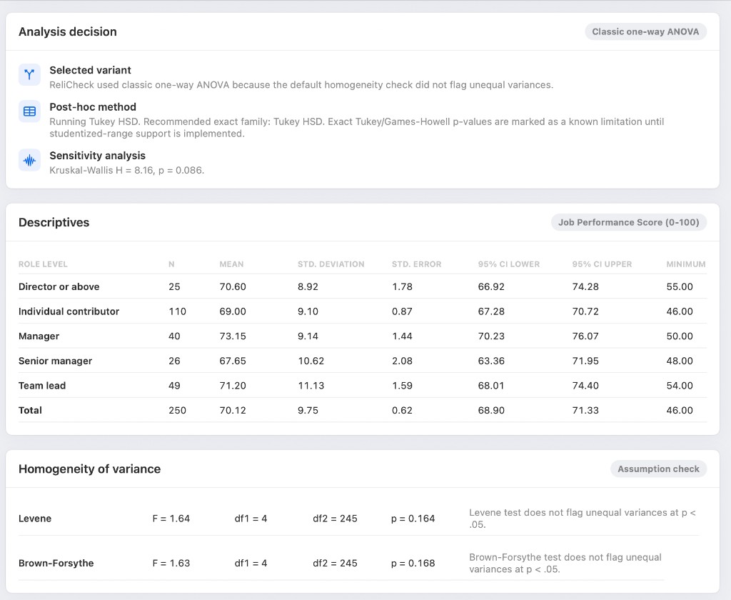
Mean is the plain average: add the scores in a group, divide by how many people are in it. Standard deviation (SD) measures how spread out those scores are around the mean; a small SD means people cluster near the average, a large SD means they are scattered. The 95% confidence interval (CI) is the believable range for the true group average, given this sample. Overlapping intervals across groups are an early hint that the groups may not really differ.
Group averages in this run
| Role Level | N | Mean | SD | 95% CI |
|---|---|---|---|---|
| Manager | 40 | 73.15 | 9.14 | 70.23–76.07 |
| Team lead | 49 | 71.20 | 11.13 | 68.01–74.40 |
| Director or above | 25 | 70.60 | 8.92 | 66.92–74.28 |
| Individual contributor | 110 | 69.00 | 9.10 | 67.28–70.72 |
| Senior manager | 26 | 67.65 | 10.62 | 63.36–71.95 |
| Total | 250 | 70.12 | 9.75 | 68.90–71.33 |
The full spread from the lowest role average to the highest is only about 5.5 points on a 0 to 100 scale (67.65 up to 73.15). Inside each role, people already vary by about 9 to 11 points, which is the SD column. The gaps between roles are smaller than the ordinary scatter within a single role. That is exactly the pattern that produces a modest F and a p-value above .05.
Individual contributors make up 110 of the 250 people. Directors number 25, senior managers 26. The groups are uneven, which statisticians call an unbalanced design. Quanta flags it as a caution, not a fatal error. The follow-up test it uses (Tukey-Kramer) handles unequal group sizes, and estimates are simply more precise for the bigger groups than the small ones.
Variance is just SD squared, another measure of spread. Classic ANOVA assumes the groups have roughly equal spread. Two tests check that: Levene and Brown-Forsythe. Here Levene p = .164 and Brown-Forsythe p = .168. Both sit above .05, so neither flags unequal spreads. Roles do not appear to differ wildly in how scattered their scores are. That clean check is why Quanta chose classic one-way ANOVA and Tukey HSD, rather than the unequal-variance versions (Welch and Games-Howell).
Decode F using the sums of squares from this run
The F you saw in Lesson 2 comes from splitting the total variation in job performance into two piles, then comparing them. This lesson opens up that arithmetic so the 1.94 stops being a black box.
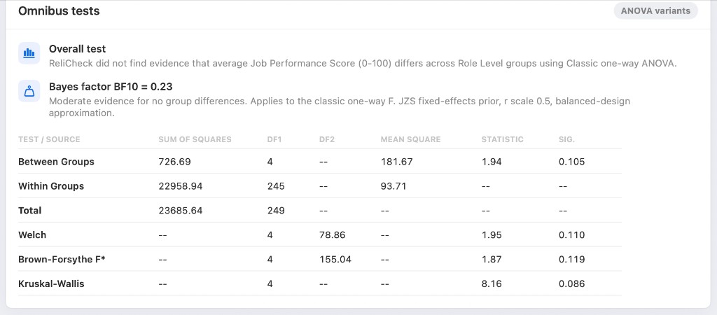
Sum of squares (SS) is a running total of variation. Between-groups SS captures how far the group averages sit from the overall average: the signal. Within-groups SS captures how far individuals sit from their own group average: the noise. Total SS is all the variation added together.
Degrees of freedom (df) is roughly the number of values free to vary; you use it to scale each pile down to a fair per-unit amount. Divide a sum of squares by its df and you get a mean square (MS). F is simply the between MS divided by the within MS: signal per unit, over noise per unit.
The numbers behind F in this run
- Between-groups SS = 726.69: the role-level pile (group averages vs. the overall average).
- Within-groups SS = 22,958.94: the person-to-person pile inside roles. The noise pile is far larger.
- Total SS = 23,685.64: all the job-performance variation in the analyzed sample.
- df between = 4 (five groups minus one); df within = 245 (250 people minus five groups).
Put the piles on a per-unit footing and divide:
The between-role mean square is only about twice the within-role mean square. For five groups and 250 people, that ratio is not extreme. The p-value of .105 follows directly: the assumption of equal role averages stays believable, because a signal only twice the size of the noise is the kind of thing luck hands you fairly often.
The other rows are a robustness chorus
Quanta also runs several backup tests. Each asks the same question a slightly different way, so you can see whether the answer holds up when you change the assumptions.
When the classic test, Welch, Brown-Forsythe, Kruskal-Wallis, and the Bayes factor all decline to declare a role effect, you are not staring at a fragile p = .049 that would flip if one assumption changed. You are looking at a stable “not much here” signal. Agreement across methods is what makes a null result trustworthy.
Post-hoc tests and effect size: where the 5.5 points go
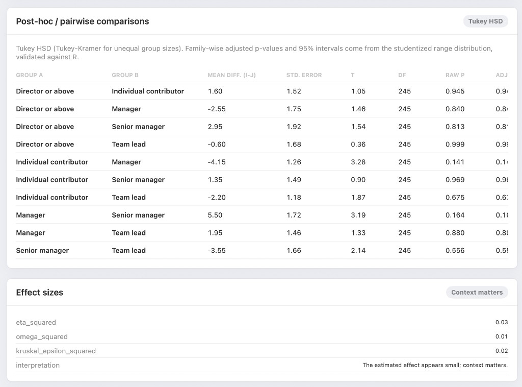
Post-hoc is Latin for “after this”. A post-hoc test runs after the omnibus ANOVA to check specific pairs of groups, and it tightens its cutoffs to account for the many comparisons, so the false-alarm rate for the whole family of pairs stays near 5%. Tukey HSD (Honestly Significant Difference) is the standard post-hoc test for this design.
What Tukey says about these roles
The biggest average gaps show up as pairs: Individual contributor vs. Manager (a 4.15-point gap) and Manager vs. Senior manager (a 5.50-point gap). On their own, those gaps carry raw p-values around .14 to .16. After Tukey adjusts for testing every pair at once, none of them clears .05. Quanta’s summary line is literal: no Tukey HSD comparison lands below p = .05.
Even if the omnibus had been significant, you would still need the pairwise table to name which roles differ. Here the omnibus did not clear .05 and the pairs agree with it. Do not invent a “Managers outperform Senior managers” headline from the raw averages alone. The averages differ; the test says that difference is within the range of luck.
What eta-squared = .03 says
Significance tells you whether a difference is more than luck. Effect size tells you how big the difference is in practical terms. Eta-squared is the share of the variation in the outcome that lines up with the grouping. Eta-squared = .03 means role level is associated with about 3% of the variation in job performance in this sample. The other 97% sits somewhere else. Two related measures, omega-squared = .01 and Kruskal epsilon-squared = .02, tell the same small story.
A non-significant F paired with a small eta-squared is one coherent story, not a contradiction. Role level is not carving job performance into distinct bands here, and even the sliver of association there is stays small. Always read both numbers. A big effect that is not significant hints at too small a sample; a significant result with a tiny effect can be real but trivial.
Warnings, report language, and the drafting helper
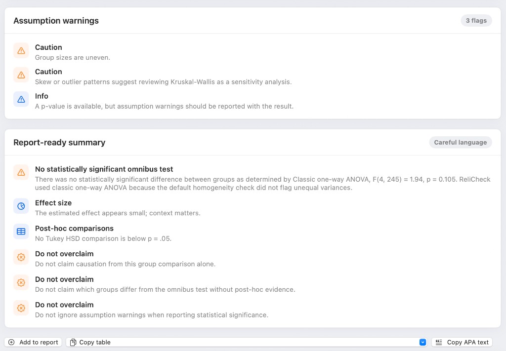
What Quanta flags here
- Uneven group sizes. Individual contributors dominate, so the Director and Senior manager estimates are noisier than the others.
- Skew or outliers, review Kruskal-Wallis. Already done (p = .086). The rank-based test did not rescue a role effect.
- Report the warnings with the p-value. One honest sentence about the imbalance belongs in the results, not buried in a footnote.
First, this design does not prove role level causes performance; it measures association in one sample. Second, you may not name a winning role pair without post-hoc support, and you do not have that support here. Third, a clean p-value sentence that skips the uneven group sizes and the Kruskal-Wallis check is incomplete. Say what you found, and say what would make it shaky.

ReliCheck Intelligence runs on your device and explains the result that Quanta already computed. It never recomputes the statistics, and it does not change any number. Treat it as a drafting aid, then edit its wording against the actual numbers and warnings above before you use it.
Exit ticket: defend what the data said
If you can answer these without looking, you understand the run, not just the menus.
In one sentence, what did Job Performance do across Role Level in this sample?
Why is F ≈ 1.94 “small” in plain terms?
What does eta-squared = .03 tell you that p = .105 does not?
Why did Quanta choose classic ANOVA and Tukey rather than Welch and Games-Howell?
A teammate wants to report “Managers scored higher than Senior managers.” What do you say?
In this Emotional Intelligence file, role level does not cleanly sort job performance. People vary a lot inside each role. Roles differ only a little at the average. The classic ANOVA, its robust backups, the rank test, the Bayes factor, the Tukey pairs, and the effect size all point the same way: little evidence of a role-level effect worth building a claim on.
Report-ready language
Use these blocks when you need manuscript-ready results wording for this worked example. They match Quanta’s report export for this run.
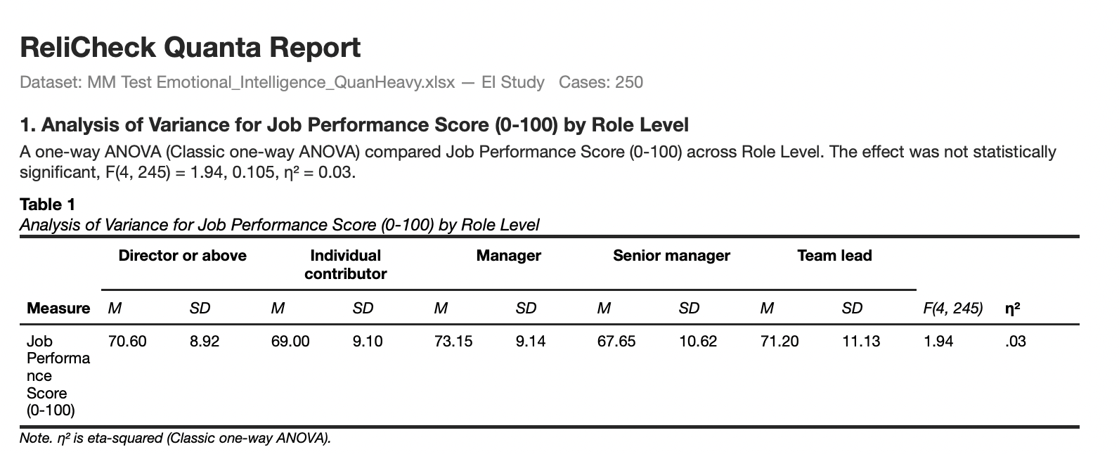
Evidence → Compare Means → One-way ANOVA. For ANCOVA, repeated measures, and factorial designs, use the separate tools under Compare Means.
Keep going
The step-by-step reference for this procedure is the one-way ANOVA page, which covers the assumption checks, the robustness tests reported beside the F, the Bayes factor, and the APA result line. Every procedure Quanta runs has one, listed on the analyses page.